
Soil survey and testing
A map of every soil property, checked against your own lab results
We survey the paddock once, place soil tests where the survey says they will tell us most, and build a predicted map of each property at every point, each one graded on soil tests it never saw.
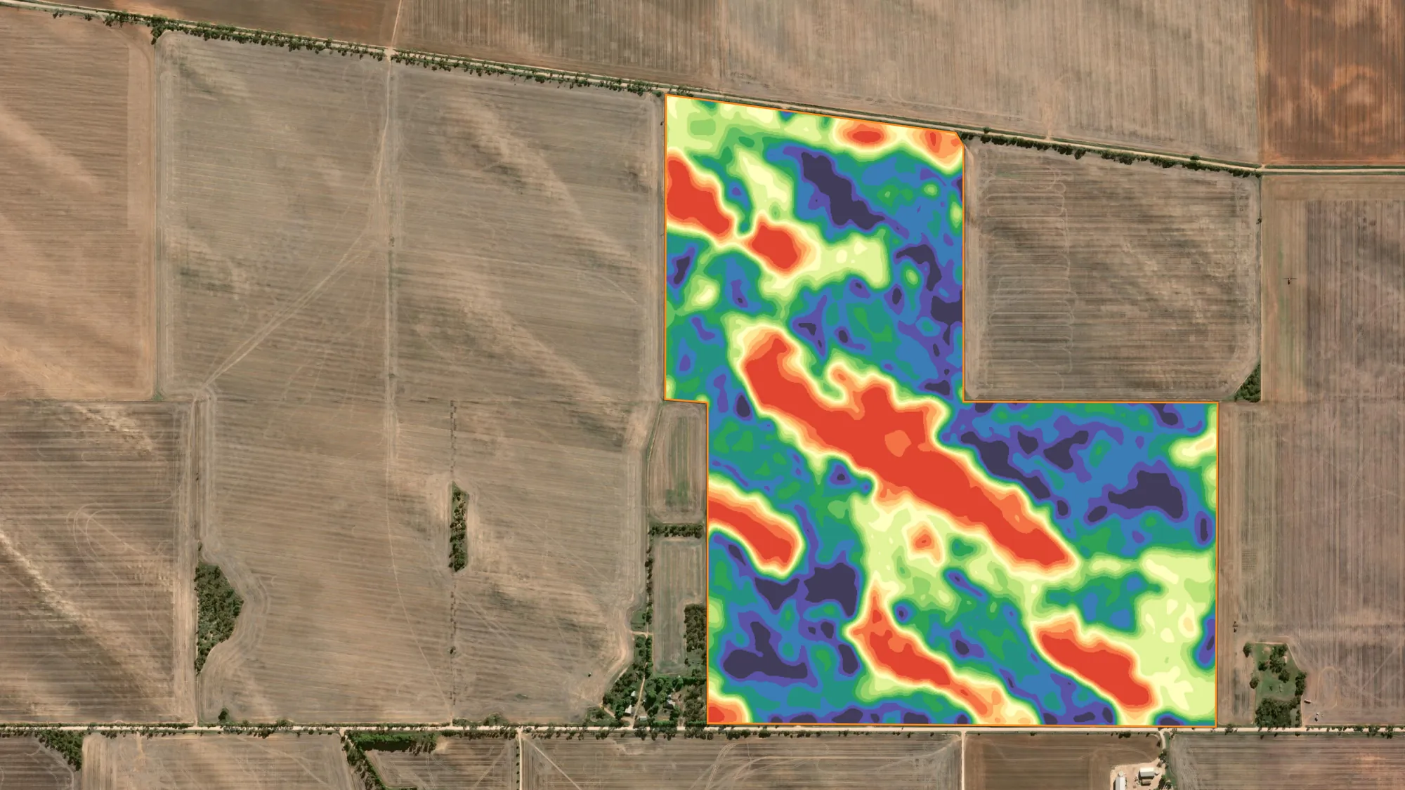
on this map0.91
On this page
On this page
Step 1
The survey: four sensors, one pass
Every soil map starts with a run across the whole paddock. Our survey sled carries a DualEM-1HS electromagnetic sensor, a four-channel gamma-ray spectrometer and RTK GPS on a 24 m swath. In one pass it logs soil conductivity at four depths, four gamma channels and centimetre-grade elevation at every point. Satellite layers come with every survey.
Electromagnetic · DualEM
Soil conductivity read at 25, 50, 80 and 160 cm: texture changes, depth to clay, salinity risk and sand-to-clay transitions, and how the soil changes with depth.
Gamma radiometrics · K, Th, U
Parent material, clay mineralogy and weathering in the top 30 cm. These are the soil-type changes that EM alone can't separate.
RTK elevation and terrain
Slope, water flow, wet spots and erosion. Landscape position explains much of the soil and yield variation in a paddock.
Satellite · Sentinel-2
Bare-earth soil colour, iron oxide and long-term NDVI, which shows how each part of the paddock has grown over many seasons.


Survey layers from four different paddocks. Imagery © Esri, Maxar.
Step 2
Targeted soil tests, not a grid
Instead of a grid, the survey layers design the soil-test plan. Cropix uses conditioned Latin hypercube sampling (cLHS), which reads every layer together and picks sites that:
- capture the full range, from low to medium to high zones;
- represent the key soil types and the transitions between them;
- avoid tight clusters or bias towards one part of the paddock;
- get the most information out of every sample.
Sites are kept off the boundary, and trees, dams and other problem areas can be drawn out before the plan is made. Fewer, better-placed samples make higher-value tests affordable, like multi-depth sampling by horizon and Deep N.
Standard test panel: pH, PBI unadjusted, Colwell P, DGT-P, Colwell K, EC 1:5, exchangeable cations and CEC. Custom panels suit every soil type, and multi-depth sampling is available.


Choosing an approach
Grid sampling or sensor-driven mapping
Both maps below show PBI across the same 110 ha paddock. The grid map can only join the dots between sample sites, so its zones are broad and smooth. The sensor-driven map uses targeted samples and the survey layers to predict PBI at every point. It follows the real soil boundaries, including the sharp band in the south-east and the strip down the centre that the grid smooths away.


Grid sampling is reasonable when
- no sensor data is available and a basic overview is enough;
- the paddock has very low soil variability;
- a quick, one-off, low-cost snapshot is all you need.
Sensor-driven mapping is the better choice when
- you want accurate maps without oversampling;
- you need tests at several depths, or an expensive test panel;
- you're building a precision ag program for years to come;
- VRA prescriptions need to stand up statistically.
EM, gamma and elevation layers stay stable for many years, so the same survey is used again as soil tests are added in later seasons. The trade-off: it needs a survey up front, the analysis takes longer, and some nutrients need more tests for an accurate model.
What you get
33 layers from four sensor streams
Each stream sees a different physical property of the paddock. Cropix then combines the raw layers into derivatives (ratios, residuals, interactions and variance), each isolating a signal no single sensor can resolve. South Australian paddocks mix shallow calcrete, sodic clay subsoils, sand hills and heavy swales, and fusing the sensors is what tells heavy clay subsoil in a wet spot from shallow rock on a slope. Those two can look identical on an NDVI map.


Maps from six different paddocks. Imagery © Esri, Maxar.
Survey and satellite
- DualEM 25 cm
- DualEM 50 cm
- DualEM 80 cm
- DualEM 160 cm
- Gamma potassium
- Gamma thorium
- Gamma uranium
- Gamma total count
- Bare earth
- Iron oxide
- NBR
- NDVI
- NDVI long-term average
- NDVI long-term P5
- NDVI long-term P50
- NDVI long-term P95
Terrain and derivatives
- Elevation
- Slope
- Landscape change
- TWI
- Plan curvature
- Profile curvature
- EC × TWI interaction
- EC depth change
- EC depth ratio
- EC mid transition
- EC profile variance
- Th–EC residual
- Th/K ratio
- ThU index
- U/K ratio
- U/Th ratio
- Constraint Index

Step 3
The regression engine
A soil test gives you the answer at one spot. A predicted layer gives you the answer everywhere, by learning how your soil tests relate to the survey layers that cover every square metre of the paddock. The engine runs hundreds to thousands of models per property and keeps the one that predicts best.
- Data checks
Lab results are matched to their GPS sites and checked before anything is modelled.
- Outliers
Samples that don't fit the paddock's pattern are flagged, so one bad sample can't skew the map.
- Layer ranking
Every layer is screened on its own against the soil property and ranked.
- Configuration
Model types and the cross-validation method are set to suit the number of samples.
- Model search
Combinations of the strongest layers are tested across eight model types.
- Results map
The winning model maps the property across the paddock, with a scatterplot and accuracy summary.

Eight model types
- Linear
- Quadratic
- Polynomial
- Random forest
- Extra trees
- Gradient boosting
- K-nearest neighbours
- Huber (outlier-robust)
The check: leave one site out
A model always fits the points it was built from. What matters is how well it predicts ground it hasn't seen, because that's what the map does across the rest of the paddock. So one soil-test site is hidden, the model is rebuilt from the others, and the hidden site is predicted as if it had never been sampled. That repeats until every site has had its turn, and the hidden-site predictions are compared with the lab. That score is the CV-R².
How accurate is a map
Every predicted map comes with three numbers. R² shows how well the model fits the soil tests it learned from. CV-R² shows how well it predicts soil tests it never saw, which is exactly what the map does everywhere you didn't sample. Cropix ranks models on CV-R², not R².
0.70 and above · Strong
The map predicts unsampled ground reliably. Ready for zoning and variable-rate prescriptions.
0.40 to 0.70 · Moderate
The broad pattern is right, but individual values are less certain. Useful for zones and for deciding where to test next.
Below 0.40 · Weak
Not enough evidence yet. More soil tests, placed where the model is least sure, are usually the fix.
Why R² alone can't be trusted
A phosphorus model built from seven soil tests reproduced all seven exactly (R² 1.00). Asked to predict a site it hadn't seen, it explained less than a third of the variation (CV-R² 0.28). The PBI model above barely drops at all, from R² 0.92 to CV-R² 0.91: hidden sites are predicted nearly as well as the ones it learned from.
LCCC checks the numbers
CV-R² checks the pattern. Lin's concordance (LCCC) checks the values, by measuring how closely predictions sit on the 1:1 line against the lab. A model can follow the trend but read consistently high or low; LCCC catches that. 1.00 is perfect agreement.
Models are tested by leaving one site out, by k-fold groups for larger sample sets, or by hiding whole blocks of the paddock at once, the strictest test that a model still works away from where it was sampled.
Predicted maps
All the survey data and every targeted soil test go into one result: a statistically backed predicted layer for each nutrient or soil property. Here are pH, PBI and phosphorus from three paddocks, each with its model, soil tests and accuracy.


Step 4
What you receive, and the prescriptions
- A predicted map for every soil property tested: pH, PBI, Colwell P, DGT-P, Colwell K, EC, cations and CEC, each at full paddock resolution instead of one value per grid cell.
- A model summary for each map: the layers used, the model type, the number of soil tests, and its R², CV-R² and LCCC.
- Predicted against measured scatterplots, so you can see where the model is strong and where it's stretched.
- The laboratory table: every result, site by site, rated against its critical value.
- Suggested management zones, ready for zone-based rates or the next round of testing.
- A PDF or PowerPoint report with every map, model summary and table.
Prescriptions are built in Cropix from any layer: a prediction map, a yield zone, a survey layer or a drone scan. Use them for variable-rate P, K, lime and gypsum, soil amelioration, and urea from protein layers, with one product or several on the same map. Zones by natural breaks, quantiles, equal interval, standard deviation or your own thresholds, exported ready for your controller. VRA maps are $75.00 per product, per map.


Step 5
Year two and beyond
The survey is a one-off. Its 33 layers describe the soil itself, so they don't expire unless the soil is physically changed by clay spreading, delving or spading. From year two the main ongoing cost is soil testing, and because the tests are targeted, fewer are needed. A grid has to be re-sampled at full density every time; here only a handful of well-placed sites are re-tested and the survey layers fill in the rest.
- Baseline survey and soil tests
A predicted map for every soil property, each graded by its CV-R².
- Adjust rates each season
Yield maps show what every part of the paddock removed, and rates are adjusted slightly to replace it.
- Re-test every 3 to 4 years
A small round of targeted tests goes back into the model against the same survey, and the maps and prescriptions are corrected.
Soil survey and test prices
Satellite layers and prediction maps come with every survey. Subscriptions and every other service are on the pricing page.
| Service | Unit | Rate (ex GST) |
|---|---|---|
| EM / gamma / elevation surveyFull proximal sensing pass. | per ha | $17.50/ha |
| Remote sensing layersNDVI, RGB, NBR, iron oxide. Included with the survey. | per ha | Free |
| Prediction maps for VRAIncluded with the survey. Zonal soil tests required. | per farm | Free |
| Zonal soil testRequires a completed survey. Minimum 10 per paddock, including 1–2 extreme spots. Varies with the test package. | per test | $95.00 |
| Multi-depth by horizonMinimum 10 per paddock. | per depth, per test | $65.00 |
| Deep N soil testMultiple depths, placed using the protein layer. | per test | $95.00 |
| Higher-resolution single test | per test | $16.00 |
| Grid soil testComprehensive analysis. Price varies by lab and test package. | per test | Variable |
Standard test: pH, PBI unadjusted, Colwell P, DGT-P, Colwell K, EC 1:5, exchangeable cations, CEC. All prices in Australian dollars, ex GST, current as at October 2026 and subject to change.